Introduction to Bulk B Cell Repertoire Analysis using the Immcantation Framework
The field of high-throughput adaptive immune receptor repertoire sequencing (AIRR-seq) has experienced significant growth in recent years, but this growth has come with considerable complexity and variety in experimental design. These complexities, combined with the high germline and somatic diversity of immunoglobulin repertoires, present analytical challenges requiring specialized methodologies. In this tutorial, we present an example pipeline for processing bulk BCR data.
The tutorial is available as a R Markdown notebook in the Immcantation repository: intro-lab.Rmd.
This tutorial covers:
V(D)J gene annotation and novel polymorphism detection
Inference of B cell clonal relationships
Diversity analysis
Lineage tree reconstruction
Mutational load profiling
Modeling of somatic hypermutation (SHM) targeting
Quantification of selection pressure
For installation of docker used in this tutorial, go to the link given below:
https://immcantation.readthedocs.io/en/latest/docker/intro.html
Software versions
Use this command to list the software versions:
versions report

## immcantation: devel
## date: 2024.01.23
##
## presto: 0.7.2
## changeo: 1.3.0
## alakazam: 1.3.0.999
## shazam: 1.2.0.999
## tigger: 1.1.0
## scoper: 1.3.0
## dowser: 2.1.0
## enchantr: 0.1.10.999
## prestor: 0.0.7
## piglet: None
## rabhit: 0.2.5
## rdi: 1.0.0
## igphyml: 2.0.0
## seurat: 5.0.1
##
## airr-py: 1.5.0
## airr-r: 1.5.0
## blast: 2.13.0
## cd-hit: 4.8.1
## igblast: 1.22.0
## muscle: 3.8.425
## phylip: 3.697
## raxml-ng: 1.2.0
## vsearch: 2.22.1
Build versions
Use this command to list the date and changesets used during the image build:
builds report

## date: 2024-01-24 07:50:57 UTC
## immcantation: 4.4.0-251-ga68604b5037a+
## presto: 0.7.2
## changeo: 1.3.0-20-g14bc8feffaaa
## alakazam: 1.2.0-85-gdfd2bff439c3+
## shazam: 1.1.2-67-gc1c6483baa5f+
## tigger: b0ad8b4f4fb9+
## rdi: d27b9067cab6+
## scoper: 1.2.0-65-gd3ee771d2b28+
## dowser: 2.0.0-19-g8c0d17173ab5+
## prestor: 0.0.8+
Example data used in the tutorial
You can download the example data from Zenodo
![]() .
It is alreday available in the container:
.
It is alreday available in the container:
/home/magus/data/input.fasta: Processed B cell receptor reads from one
healthy donor (PGP1) 3 weeks after flu vaccination (Laserson et
al. (2014))
As part of the processing, each sequence has been annotated with the isotype.
This step is not a part of the tutorial, but you can learn how to do it here.
head /home/magus/data/input.fasta

## >seq1|ISOTYPE=IGHM
## nnnnnnnnnnnnnnnnnnnnnnnagtgtcaggtgcagctggtggagctggggagcgtggt
## ccagcctgggaggccctgagtctctcctgtgcagcctctggattcaccttcagtctctat
## gctatgcactgggtccgccaggctccaggcaaggggctggagtgggtggcagttatatca
## tatcatgtaagcagtaaatactacgcagactccgtgaagggccgattcaccatctccaga
## gacaattccaagaacacgctgtatctgcaaatgaacagcctgagagctgaggacacggct
## gtgtattactgtgcgagagggccctatagtactggttattactacgagcttgactactgg
## ggccagggaacgctcggtcacccgtctcctcacgggtagtgcatccgccccaaccc
## >seq2|ISOTYPE=IGHM
## nnnnnnnnnnnnnnnnnntgtcccaggtgcagctgcaggagtcgggcccaggactggtga
Reference germlines
The container has human and mouse reference V(D)J germline genes from
IMGT (/usr/local/share/germlines/imgt) and the corresponding IgBLAST
databases (/usr/local/share/igblast) for these germline repertoires.
The training container also contains a modified version of these
databases where allele IGHV3-20*04 has been removed, to be rediscovered
by TIgGER. The modified databases are in
/usr/local/share/germlines/imgt_test_tigger and
/usr/local/share/igblast_test_tigger.
ls /usr/local/share/germlines/imgt

## IMGT.yaml
## human
## mouse
## rabbit
## rat
## rhesus_monkey

ls /usr/local/share/igblast

## database
## fasta
## internal_data
## optional_file
V(D)J gene annotation
The first step in the analysis of processed reads (input.fasta) is to
annotate each read with its germline V(D)J gene alleles and to identify
relevant sequence structure such as the CDR3 sequence. Immcantation
provides tools to read the output of many popular V(D)J assignment
tools, including IMGT/HighV-QUEST and
IgBLAST.
Here, we will use IgBLAST. Change-O provides a wrapper script
(AssignGenes.py) to run IgBLAST using the reference V(D)J germline
sequences in the container.
A test with 200 sequences
It is often useful to prototype analysis pipelines using a small subset
of sequences. For a quick test of Change-O’s V(D)J assignment tool, use
SplitSeq.py to extract 200 sequences from input.fasta, then assign
the V(D)J genes with AssignGenes.py.
mkdir -p results/igblast
SplitSeq.py sample -n 200 --outdir results --fasta -s /home/magus/data/input.fasta

##      START> SplitSeq
##    COMMAND> sample
##       FILE> input.fasta
## MAX_COUNTS> 200
##      FIELD> None
##     VALUES> None
##
## PROGRESS> 13:43:20 |Reading files            | 0.0 minPROGRESS> 13:43:20 |Done                     | 0.0 min
##
## PROGRESS> 13:43:20 |Sampling n=200           | 0.0 minPROGRESS> 13:43:20 |Done                     | 0.0 min
##
## MAX_COUNT> 200
##   SAMPLED> 200
##    OUTPUT> input_sample1-n200.fasta
##
## END> SplitSeq
AssignGenes.py performs V(D)J assignment with IgBLAST.
It requires the input sequences (
-s) and a reference germlines database (-b). In this case, we use the germline database already available in the container.The organism is specified with
--organismand the type of receptor with--loci(igfor the B cell receptor).Use
--format blastto specify that the results should be in thefmt7format.Improved computational speed can be achieved by specifying the number of processors with
--nproc.
AssignGenes.py igblast -s results/input_sample1-n200.fasta \
-b /usr/local/share/igblast_test_tigger --organism human --loci ig \
--format blast --outdir results/igblast --nproc 8

##    START> AssignGenes
##  COMMAND> igblast
##  VERSION> 1.22.0
##     FILE> input_sample1-n200.fasta
## ORGANISM> human
##     LOCI> ig
##    NPROC> 8
##
## PROGRESS> 13:43:22 |Running IgBLAST          | 0.0 minPROGRESS> 13:43:24 |Done                     | 0.0 min
##
##   PASS> 200
## OUTPUT> input_sample1-n200_igblast.fmt7
##    END> AssignGenes
V(D)J assignment using all the data
To run the command on all of the data, modify it to change the input
file (-s) to the full data set. Please note that this may take some
time to finish running.
AssignGenes.py igblast -s /home/magus/data/input.fasta \
-b /usr/local/share/igblast_test_tigger --organism human --loci ig \
--format blast --outdir results/igblast --nproc 8

##    START> AssignGenes
##  COMMAND> igblast
##  VERSION> 1.22.0
##     FILE> input.fasta
## ORGANISM> human
##     LOCI> ig
##    NPROC> 8
##
## PROGRESS> 13:43:27 |Running IgBLAST          | 0.0 minPROGRESS> 14:01:27 |Done                     | 18.0 min
##
##   PASS> 91010
## OUTPUT> input_igblast.fmt7
##    END> AssignGenes
Data standardization using Change-O
Once the V(D)J annotation is finished, the IgBLAST results are parsed into a standardized format suitable for downstream analysis. All tools in the Immcantation framework use this format, which allows for interoperability and provides flexibility when designing complex workflows.
In this example analysis, the fmt7 results from IgBLAST are converted
into the
AIRR
format, a tabulated text file with one sequence per row. Columns provide
the annotation for each sequence using standard column names as
described here:
https://docs.airr-community.org/en/latest/datarep/rearrangements.html.
Generate a standardized database file
The command line tool MakeDb.py igblast requires the original input
sequence fasta file (-s) that was passed to the V(D)J annotation tool,
as well as the V(D)J annotation results (-i). The argument
--format airr specifies that the results should be converted into the
AIRR format. The path to the reference germlines is provided by -r.
mkdir -p results/changeo
MakeDb.py igblast \
-s /home/magus/data/input.fasta -i results/igblast/input_igblast.fmt7 \
--format airr \
-r /usr/local/share/germlines/imgt_test_tigger/human/vdj/ --outdir results/changeo \
--outname data

##          START> MakeDB
##        COMMAND> igblast
##   ALIGNER_FILE> input_igblast.fmt7
##       SEQ_FILE> input.fasta
##        ASIS_ID> False
##     ASIS_CALLS> False
##       VALIDATE> strict
##       EXTENDED> False
## INFER_JUNCTION> False
##
## PROGRESS> 14:01:27 |Loading files       | 0.0 minPROGRESS> 14:01:28 |Done                | 0.0 min
##
## PROGRESS> 14:01:28 |                    |   0% (     0) 0.0 minPROGRESS> 14:01:31 |#                   |   5% ( 4,551) 0.0 minPROGRESS> 14:01:34 |##                  |  10% ( 9,102) 0.1 minPROGRESS> 14:01:36 |###                 |  15% (13,653) 0.1 minPROGRESS> 14:01:39 |####                |  20% (18,204) 0.2 minPROGRESS> 14:01:42 |#####               |  25% (22,755) 0.2 minPROGRESS> 14:01:44 |######              |  30% (27,306) 0.3 minPROGRESS> 14:01:46 |#######             |  35% (31,857) 0.3 minPROGRESS> 14:01:49 |########            |  40% (36,408) 0.3 minPROGRESS> 14:01:52 |#########           |  45% (40,959) 0.4 minPROGRESS> 14:01:54 |##########          |  50% (45,510) 0.4 minPROGRESS> 14:01:56 |###########         |  55% (50,061) 0.5 minPROGRESS> 14:01:59 |############        |  60% (54,612) 0.5 minPROGRESS> 14:02:01 |#############       |  65% (59,163) 0.5 minPROGRESS> 14:02:03 |##############      |  70% (63,714) 0.6 minPROGRESS> 14:02:06 |###############     |  75% (68,265) 0.6 minPROGRESS> 14:02:08 |################    |  80% (72,816) 0.7 minPROGRESS> 14:02:10 |#################   |  85% (77,367) 0.7 minPROGRESS> 14:02:13 |##################  |  90% (81,918) 0.7 minPROGRESS> 14:02:15 |################### |  95% (86,469) 0.8 minPROGRESS> 14:02:17 |####################| 100% (91,010) 0.8 min
##
## OUTPUT> data_db-pass.tsv
##   PASS> 87785
##   FAIL> 3225
##    END> MakeDb
Subset the data to include productive heavy chain sequences
We next filter the data from the previous step to include only productive sequences from the heavy chain. The determination of whether a sequence is productive (or not) is provided by the V(D)J annotation software.
ParseDb.py select finds the rows in the file -d for which the column
productive (specified with -f) contains the values T or TRUE
(specified by -u). The prefix data_p will be used in the name of the
output file (specified by --outname).
ParseDb.py select -d results/changeo/data_db-pass.tsv \
-f productive -u T --outname data_p

##   START> ParseDb
## COMMAND> select
##    FILE> data_db-pass.tsv
##  FIELDS> productive
##  VALUES> T
##   REGEX> False
##
## PROGRESS> 14:02:18 |                    |   0% (     0) 0.0 minPROGRESS> 14:02:18 |#                   |   5% ( 4,390) 0.0 minPROGRESS> 14:02:18 |##                  |  10% ( 8,780) 0.0 minPROGRESS> 14:02:18 |###                 |  15% (13,170) 0.0 minPROGRESS> 14:02:18 |####                |  20% (17,560) 0.0 minPROGRESS> 14:02:19 |#####               |  25% (21,950) 0.0 minPROGRESS> 14:02:19 |######              |  30% (26,340) 0.0 minPROGRESS> 14:02:19 |#######             |  35% (30,730) 0.0 minPROGRESS> 14:02:19 |########            |  40% (35,120) 0.0 minPROGRESS> 14:02:19 |#########           |  45% (39,510) 0.0 minPROGRESS> 14:02:19 |##########          |  50% (43,900) 0.0 minPROGRESS> 14:02:19 |###########         |  55% (48,290) 0.0 minPROGRESS> 14:02:19 |############        |  60% (52,680) 0.0 minPROGRESS> 14:02:20 |#############       |  65% (57,070) 0.0 minPROGRESS> 14:02:20 |##############      |  70% (61,460) 0.0 minPROGRESS> 14:02:20 |###############     |  75% (65,850) 0.0 minPROGRESS> 14:02:20 |################    |  80% (70,240) 0.0 minPROGRESS> 14:02:20 |#################   |  85% (74,630) 0.0 minPROGRESS> 14:02:20 |##################  |  90% (79,020) 0.0 minPROGRESS> 14:02:20 |################### |  95% (83,410) 0.0 minPROGRESS> 14:02:20 |####################| 100% (87,785) 0.0 min
##
##    OUTPUT> data_p_parse-select.tsv
##   RECORDS> 87785
##  SELECTED> 64968
## DISCARDED> 22817
##       END> ParseDb
Next, we filter the data to include only heavy chain sequences.
ParseDb.py select finds the rows in the file -d from the previous
step for which the column v_call (specified with -f) contains
(pattern matching specified by --regex) the word IGHV (specified by
-u). The prefix data_ph (standing for productive and heavy) will be
used in the name of the output file (specified by --outname) to
indicate that this file contains productive (p) heavy (h) chain sequence
data.
ParseDb.py select -d results/changeo/data_p_parse-select.tsv \
-f v_call -u IGHV --regex --outname data_ph

##   START> ParseDb
## COMMAND> select
##    FILE> data_p_parse-select.tsv
##  FIELDS> v_call
##  VALUES> IGHV
##   REGEX> True
##
## PROGRESS> 14:02:21 |                    |   0% (     0) 0.0 minPROGRESS> 14:02:21 |#                   |   5% ( 3,249) 0.0 minPROGRESS> 14:02:22 |##                  |  10% ( 6,498) 0.0 minPROGRESS> 14:02:22 |###                 |  15% ( 9,747) 0.0 minPROGRESS> 14:02:22 |####                |  20% (12,996) 0.0 minPROGRESS> 14:02:22 |#####               |  25% (16,245) 0.0 minPROGRESS> 14:02:22 |######              |  30% (19,494) 0.0 minPROGRESS> 14:02:22 |#######             |  35% (22,743) 0.0 minPROGRESS> 14:02:22 |########            |  40% (25,992) 0.0 minPROGRESS> 14:02:22 |#########           |  45% (29,241) 0.0 minPROGRESS> 14:02:22 |##########          |  50% (32,490) 0.0 minPROGRESS> 14:02:23 |###########         |  55% (35,739) 0.0 minPROGRESS> 14:02:23 |############        |  60% (38,988) 0.0 minPROGRESS> 14:02:23 |#############       |  65% (42,237) 0.0 minPROGRESS> 14:02:23 |##############      |  70% (45,486) 0.0 minPROGRESS> 14:02:23 |###############     |  75% (48,735) 0.0 minPROGRESS> 14:02:23 |################    |  80% (51,984) 0.0 minPROGRESS> 14:02:23 |#################   |  85% (55,233) 0.0 minPROGRESS> 14:02:23 |##################  |  90% (58,482) 0.0 minPROGRESS> 14:02:24 |################### |  95% (61,731) 0.0 minPROGRESS> 14:02:24 |####################| 100% (64,968) 0.0 min
##
##    OUTPUT> data_ph_parse-select.tsv
##   RECORDS> 64968
##  SELECTED> 64968
## DISCARDED> 0
##       END> ParseDb
Load libraries and read in the data
After loading the libraries needed, the process is started by using
readChangeoDb to read the tabulated data generated in the previous
step.
suppressPackageStartupMessages(library(airr))
suppressPackageStartupMessages(library(alakazam))
suppressPackageStartupMessages(library(dplyr))
suppressPackageStartupMessages(library(ggplot2))
suppressPackageStartupMessages(library(tigger))

dir.create(file.path("results", "tigger"))

## Warning in dir.create(file.path("results", "tigger")): 'results/tigger' already
## exists

db <- read_rearrangement(file.path("results", "changeo",
                                   "data_ph_parse-select.tsv"))
colnames(db) # show the column names in the database

##  [1] "sequence_id"        "sequence"           "rev_comp"
##  [4] "productive"         "v_call"             "d_call"
##  [7] "j_call"             "sequence_alignment" "germline_alignment"
## [10] "junction"           "junction_aa"        "v_cigar"
## [13] "d_cigar"            "j_cigar"            "stop_codon"
## [16] "vj_in_frame"        "locus"              "c_call"
## [19] "junction_length"    "np1_length"         "np2_length"
## [22] "v_sequence_start"   "v_sequence_end"     "v_germline_start"
## [25] "v_germline_end"     "d_sequence_start"   "d_sequence_end"
## [28] "d_germline_start"   "d_germline_end"     "j_sequence_start"
## [31] "j_sequence_end"     "j_germline_start"   "j_germline_end"
## [34] "isotype"
Remove sequences with many Ns using filterN
Bulk BCR data in general includes ambiguous nucleotides (Ns), and we will remove those low-quality sequences with many Ns
# Source helper function also available here:
# https://bitbucket.org/kleinstein/immcantation/src/master/training/assets/filterN.R
source("assets/filterN.R")

# Identify sequences with at least 20 Ns or continuous 15 Ns in the v_region
v_n_stretches_plot <- filterN(db, "sequence_alignment",
                                  start=1, end=312,
                                  max_n=20, max_n_stretch = 15,
                                  label="v_region",
                                  plot=TRUE)

v_region_n_pass <- v_n_stretches_plot$db_pass
# number of sequences before filtering N
dim(db)

## [1] 64968    34

db = db[which(v_region_n_pass),]
# number of sequences after filtering N
dim(db)

## [1] 64968    34
Genotyping and discovery of novel V gene alleles with TIgGER
V(D)J assignment is a key step in analyzing repertoires and is done by matching the sequences against a database of known V(D)J alleles. However, current databases are incomplete and this process will fail for sequences that utilize previously undetected alleles. Some assignments may also occur to genes which are not carried by the individual. The TIgGER R package infers subject-specific V genotypes (including novel alleles), then uses the results to improve the V gene annotations.
readIgFasta loads the reference V germline genes that were used in the
V(D)J assignment (in this case the sequences in the Immcantation
container).
ighv <- readIgFasta(file.path("", "usr", "local", "share", "germlines",
                              "imgt_test_tigger", "human", "vdj",
                              "imgt_human_IGHV.fasta"))
ighv[1] # show the first germline

##                                                                                                                                                                                                                                                                                                                        IGHV1-18*01
## "CAGGTTCAGCTGGTGCAGTCTGGAGCT...GAGGTGAAGAAGCCTGGGGCCTCAGTGAAGGTCTCCTGCAAGGCTTCTGGTTACACCTTT............ACCAGCTATGGTATCAGCTGGGTGCGACAGGCCCCTGGACAAGGGCTTGAGTGGATGGGATGGATCAGCGCTTAC......AATGGTAACACAAACTATGCACAGAAGCTCCAG...GGCAGAGTCACCATGACCACAGACACATCCACGAGCACAGCCTACATGGAGCTGAGGAGCCTGAGATCTGACGACACGGCCGTGTATTACTGTGCGAGAGA"
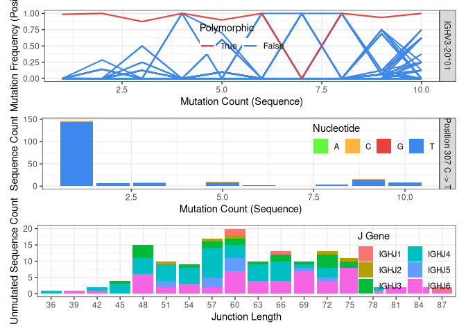
Identify potentially novel V gene alleles
For each V gene allele, findNovelAlleles analyzes the sequences that
were assigned the allele and evaluates the apparent mutation frequency
at each position as a function of sequence-wide mutation counts.
Positions that contain polymorphisms (rather than somatic
hypermutations) will exhibit a high apparent mutation frequency even
when the sequence-wide mutation count is low.
In this example, TIgGER finds one novel V gene allele.
nv <- findNovelAlleles(db, germline_db = ighv, nproc = 8) # find novel alleles

selectNovel(nv) # show novel alleles

##   germline_call                note polymorphism_call nt_substitutions
## 1   IGHV3-20*01 Novel allele found! IGHV3-20*01_C307T           307C>T
## 2   IGHV3-20*03 Novel allele found!  IGHV3-20*03_T68G            68T>G
##                                                                                                                                                                                                                                                                                                                                                                                                                                                                                                                                                                                             novel_imgt
## 1                                                                                                                                                                                                                                                                     GAGGTGCAGCTGGTGGAGTCTGGGGGA...GGTGTGGTACGGCCTGGGGGGTCCCTGAGACTCTCCTGTGCAGCCTCTGGATTCACCTTT............GATGATTATGGCATGAGCTGGGTCCGCCAAGCTCCAGGGAAGGGGCTGGAGTGGGTCTCTGGTATTAATTGGAAT......GGTGGTAGCACAGGTTATGCAGACTCTGTGAAG...GGCCGATTCACCATCTCCAGAGACAACGCCAAGAACTCCCTGTATCTGCAAATGAACAGTCTGAGAGCCGAGGACACGGCCTTGTATTACTGTGCGAGAGA
## 2 GAGGTGCAGCTGGTGGAGTCTGGGGGA...GGTGTGGTACGGCCTGGGGGGTCCCTGAGACTCTCCTGTGCAGCCTCTGGATTCACCTTT............GATGATTATGGCATGAGCTGGGTCCGCCAAGCTCCAGGGAAGGGGCTGGAGTGGGTCTCTGGTATTAATTGGAAT......GGTGGTAGCACAGGTTATGCAGACTCTGTGAAG...GGCCGATTCACCATCTCCAGAGACAACGCCAAGAACTCCCTGTATCTGCAAATGAACAGTCTGAGAGCCGAGGACACGGCCTTGTATTACTGTGCGAGAGACTCTCCTGTGCAGCCTCTGGATTCACCTTT............GATGATTATGGCATGAGCTGGGTCCGCCAAGCTCCAGGGAAGGGGCTGGAGTGGGTCTCTGGTATTAATTGGAAT......GGTGGTAGCACAGGTTATGCAGACTCTGTGAAG...GGCCGATTCACCATCTCCAGAGACAACGCCAAGAACTCCCTGTATCTGCAAATGAACAGTCTGAGAGCCGAGGACACGGCCTTGTATTACTGTGCGAGAGA
##   novel_imgt_count novel_imgt_unique_j novel_imgt_unique_cdr3
## 1              161                   6                    145
## 2              161                   6                    145
##   perfect_match_count perfect_match_freq germline_call_count germline_call_freq
## 1                 144          0.4784053                 301              0.005
## 2                 167          0.5901060                 283              0.004
##   mut_min mut_max mut_pass_count
## 1       1      10            202
## 2       1      10            222
##                                                                                                                                                                                                                                                                                                                                                                                                                                                                                                                                                                                          germline_imgt
## 1                                                                                                                                                                                                                                                                     GAGGTGCAGCTGGTGGAGTCTGGGGGA...GGTGTGGTACGGCCTGGGGGGTCCCTGAGACTCTCCTGTGCAGCCTCTGGATTCACCTTT............GATGATTATGGCATGAGCTGGGTCCGCCAAGCTCCAGGGAAGGGGCTGGAGTGGGTCTCTGGTATTAATTGGAAT......GGTGGTAGCACAGGTTATGCAGACTCTGTGAAG...GGCCGATTCACCATCTCCAGAGACAACGCCAAGAACTCCCTGTATCTGCAAATGAACAGTCTGAGAGCCGAGGACACGGCCTTGTATCACTGTGCGAGAGA
## 2 GAGGTGCAGCTGGTGGAGTCTGGGGGA...GGTGTGGTACGGCCTGGGGGGTCCCTGAGACTCTCCTTTGCAGCCTCTGGATTCACCTTT............GATGATTATGGCATGAGCTGGGTCCGCCAAGCTCCAGGGAAGGGGCTGGAGTGGGTCTCTGGTATTAATTGGAAT......GGTGGTAGCACAGGTTATGCAGACTCTGTGAAG...GGCCGATTCACCATCTCCAGAGACAACGCCAAGAACTCCCTGTATCTGCAAATGAACAGTCTGAGAGCCGAGGACACGGCCTTGTATTACTGTGCGAGAGACTCTCCTGTGCAGCCTCTGGATTCACCTTT............GATGATTATGGCATGAGCTGGGTCCGCCAAGCTCCAGGGAAGGGGCTGGAGTGGGTCTCTGGTATTAATTGGAAT......GGTGGTAGCACAGGTTATGCAGACTCTGTGAAG...GGCCGATTCACCATCTCCAGAGACAACGCCAAGAACTCCCTGTATCTGCAAATGAACAGTCTGAGAGCCGAGGACACGGCCTTGTATTACTGTGCGAGAGA
##   germline_imgt_count pos_min pos_max y_intercept y_intercept_pass snp_pass
## 1                  44       1     312       0.125                1      196
## 2                   0       1     312       0.125                1      222
##   unmutated_count unmutated_freq unmutated_snp_j_gene_length_count
## 1             144      0.4784053                                52
## 2             167      0.5901060                                54
##   snp_min_seqs_j_max_pass alpha min_seqs j_max min_frac
## 1                       1  0.05       50  0.15     0.75
## 2                       1  0.05       50  0.15     0.75
The function plotNovel helps visualize the supporting evidence for
calling the novel V gene allele. The mutation frequency of the position
that is predicted to contain a polymorphism is highlighted in red. In
this case, the position contains a high number of apparent mutations for
all sequence-wide mutation counts (top panel).
By default, findNovelAlleles uses several additional filters to avoid
false positive allele calls. For example, to avoid calling novel alleles
resulting from clonally-related sequences, TIgGER requires that
sequences perfectly matching the potential novel allele be found in
sequences with a diverse set of J genes and a range of junction lengths.
This can be observed in the bottom panel.
plotNovel(db, selectNovel(nv)[1, ]) # visualize the novel allele(s)
Genotyping, including novel V gene alleles
The next step is to infer the subject’s genotype and use this to improve the V gene calls.
inferGenotype uses a frequency-based method to determine the genotype.
For each V gene, it finds the minimum set of alleles that can explain a
specified fraction of each gene’s calls. The most commonly observed
allele of each gene is included in the genotype first, then the next
most common allele is added until the desired fraction of sequence
annotations can be explained.
Immcantation also includes other methods for inferring subject-specific
genotypes (inferGenotypeBayesian).
gt <- inferGenotype(db, germline_db = ighv, novel = nv)

# save genotype inf .fasta format to be used later with dowser::createGermlines
gtseq <- genotypeFasta(gt, ighv, nv)
writeFasta(gtseq, file.path("results", "tigger", "v_genotype.fasta"))

gt %>% arrange(total) %>% slice(1:3) # show the first 3 rows

##       gene alleles counts total note
## 1  IGHV2-5   02,01  58,48   106
## 2 IGHV3-49   04,05  77,39   116
## 3 IGHV3-11   01,04  85,53   138
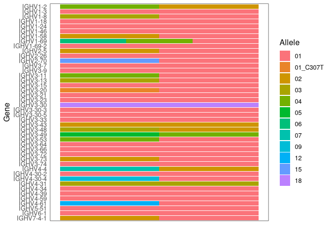
The individual’s genotype can be visualized with plotGenotype. Each
row is a gene, with colored cells indicating each of the alleles for
that gene that are included in the inferred genotype.
plotGenotype(gt) # genotyping including novel V gene alleles
Reassign V gene allele annotations
Some of the V gene calls may use genes that are not part of the
subject-specific genotype inferred by TIgGER. These gene calls can be
corrected with reassignAlleles. Mistaken allele calls can arise, for
example, from sequences which by chance have been mutated to look like
another allele. reassignAlleles saves the corrected calls in a new
column, v_call_genotyped.
With write_rearrangement the updated data is saved as a tabulated file
for use in the following steps.
db <- reassignAlleles(db, gtseq)

# show some of the corrected gene calls
db %>%
  dplyr::filter(v_call != v_call_genotyped) %>%
  sample_n(3) %>%
  select(v_call, v_call_genotyped)

## # A tibble: 3 x 2
##   v_call                      v_call_genotyped
##   <chr>                       <chr>
## 1 IGHV4-30-4*09,IGHV4-31*03   IGHV4-30-4*09
## 2 IGHV3-7*01,IGHV3-7*03       IGHV3-7*01
## 3 IGHV4-30-2*07,IGHV4-30-4*01 IGHV4-30-2*07

write_rearrangement(db, file.path("results", "tigger", "data_ph_genotyped.tsv"))
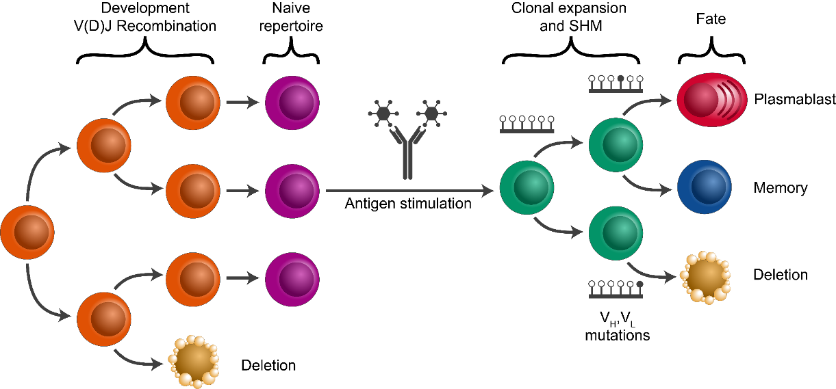
Clonal diversity analysis
Goal: Partition (cluster) sequences into clonally related lineages. Each lineage is a group of sequences that came from the same original naive cell.
Summary of the key steps: * Determine clonal clustering threshold:
sequences which are under this cut-off are clonally related. * Assign
clonal groups: add an annotation (clone_id) that can be used to
identify a group of sequences that came from the same original naive
cell. * Reconstruct germline sequences: figure out the germline
sequence of the common ancestor, before mutations are introduced during
clonal expansion and SMH. * Analyze clonal diversity: number and size
of clones? any expanded clones?
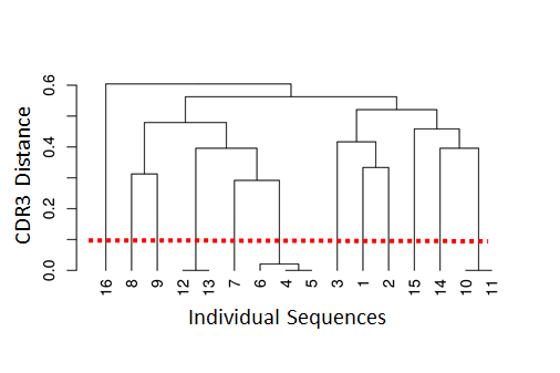
Clonal assignment using the CDR3 as a fingerprint
Clonal relationships can be inferred from sequencing data. Hierarchical clustering is a widely used method for identify clonally related sequences. This method requires a measure of distance between pairs of sequences and a choice of linkage to define the distance between groups of sequences. Since the result will be a tree, a threshold to cut the hierarchy into discrete clonal groups is also needed.
The figure below shows a tree and the chosen threshold (red dotted line). Sequences which have a distance under this threshold are considered to be part of the same clone (i.e., clonally-related) whereas sequences which have distance above this threshold are considered to be part of independent clones (i.e., not clonally related).
shazam provides methods to calculate the distance between sequences
and find an appropriate distance threshold for each dataset
(distToNearest and findThreshold). The threshold can be determined
by analyzing the distance to the nearest distribution. This is the set
of distances between each sequence and its closest non-identical
neighbor.
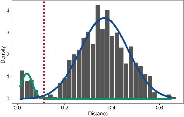
The figure below shows the distance-to-nearest distribution for a
repertoire. Typically, the distribution is bimodal. The first mode (on
the left) represents sequences that have at least one clonal relative in
the dataset, while the second mode (on the right) is representative of
the sequences that do not have any clonal relatives in the data
(sometimes called “singletons”). A reasonable threshold will separate
these two modes of the distribution. In this case, it is easy to
manually determine a threshold as a value intermediate between the two
modes. However, findThreshold can be used to automatically find the
threshold.
Setting the clonal distance threshold with SHazaM
We first split sequences into groups that share the same V and J gene
assignments and that have the same junction (or equivalently CDR3)
length. This is based on the assumption that members of a clone will
share all of these properties. distToNearest performs this grouping
step, then counts the number of mismatches in the junction region
between all pairs of sequences in each group and returns the smallest
non-zero value for each sequence. At the end of this step, a new column
(dist_nearest) which contains the distances to the closest
non-identical sequence in each group will be added to db.
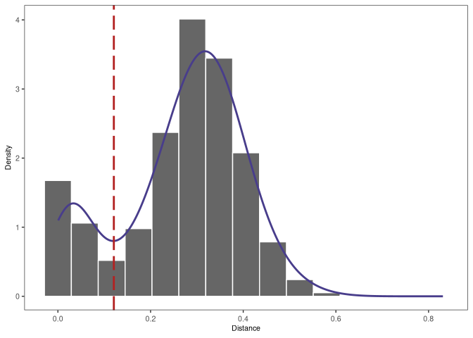
findThreshold uses the distribution of distances calculated in the
previous step to determine an appropriate threshold for the dataset.
This can be done using either a density or mixture based method. The
function plot can be used to visualize the distance-to-nearest
distribution and the threshold.
# get the distance to nearest neighbors
suppressPackageStartupMessages(library(shazam))
db <- distToNearest(db, model = "ham", normalize = "len",
                    vCallColumn = "v_call_genotyped", nproc = 4)

# determine the threshold
threshold <- findThreshold(db$dist_nearest, method = "density")
thr <- round(threshold@threshold, 2)
thr

## [1] 0.12

plot(threshold) # plot the distribution
Advanced method: Spectral-based clonal clustering (SCOPer)
In some datasets, the distance-to-nearest distribution may not be
bimodal and findThreshold may fail to determine the distance
threshold. In these cases, spectral clustering with an adaptive
threshold to determine the local sequence neighborhood may be used. This
can be done with functions from the SCOPer R
package.
Clonal assignment
Once a threshold is decided, the function hierarchicalClones from the
SCOPer R package performs the clonal
assignment. There are some arguments that usually need to be specified:
* model: the distance metric used in distToNearest * normalize:
type of normalization used in distToNearest * threshold: the
cut-off from findThreshold
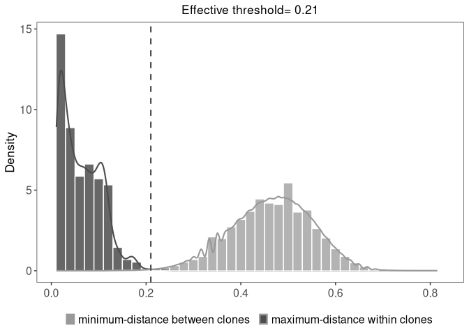
At the end of this step, the output file will have an additional column
(clone_id) that provides an identifier for each sequence to indicate
which clone it belongs to (i.e., sequences that have the same identifier
are clonally-related). Note that these identifiers are only unique to
the dataset used to carry out the clonal assignments.
suppressPackageStartupMessages(library(scoper))
# Clonal assignment using hierarchical clustering
results <- hierarchicalClones(db, threshold=thr, v_call="v_call_genotyped")

# Plot a histogram of inter and intra clonal distances
plot(results, binwidth=0.02)
Dowser: lineage reconstruction
B cell repertoires often consist of hundreds to thousands of separate
clones. A clonal lineage recapitulates the ancestor-descendant
relationships between clonally-related B cells and uncovering these
relationships can provide insights into affinity maturation. The R
package dowser offers multiple ways to build B cell phylogenetic
trees. Before performing lineage reconstruction, some preprocessing in
needed.
Create germlines
The goal is to reconstruct the sequence of the unmutated ancestor of
each clone. We use a reference database of known alleles
(IMGT). Because it is very difficult to
accurately infer the D region and the junction region for BCR sequences,
we mask this region with N.
Before B cell lineage trees can be built, it is necessary to construct the unmutated germline sequence for each B cell clone. Typically the IGH D segment is masked because the junction region of heavy chains often cannot be reliably reconstructed. Note that occasionally errors are thrown for some clones - this is typical and usually results in those clones being excluded.
In the example below, we read in the IMGT germline references from our Docker container. If you’re using a local installation, you can download the most up-to-date reference genome by cloning the Immcantation repository and running the script:
# Retrieve reference genome with the script fetch_imgtdb.sh.
# It will create directories where it is run
git clone https://bitbucket.org/kleinstein/immcantation.git
./immcantation/scripts/fetch_imgtdb.sh
And passing "human/vdj/" to the readIMGT function.
# read in IMGT data if downloaded on your own (above)
# and update `dir` to use the path to your `human/vdj` folder
# references <- readIMGT(dir = "human/vdj/")

# read in IMGT files in the Docker container
references <- dowser::readIMGT(dir = "/usr/local/share/germlines/imgt/human/vdj")

## [1] "Read in 1181 from 17 fasta files"

# reconstruct germlines
results@db <- dowser::createGermlines(results@db, references, nproc = 1)
Format clones
In the rearrangement table, each row corresponds to a sequence, and each
column is information about that sequence. We will create a new data
structure, where each row is a clonal cluster, and each column is
information about that clonal cluster. The function formatClones
performs this processing and has options that are relevant to determine
how the trees can be built and visualized. For example, traits
determines the columns from the rearrangement data that will be included
in the clones object, and will also be used to determine the
uniqueness of the sequences, so they are not collapsed.
# make clone objects with aligned, processed sequences
# collapse identical sequences unless differ by trait
# add up duplicate_count column for collapsed sequences
# store day, gex_annotation
# discard clones with < 5 distinct sequences
clones <- dowser::formatClones(results@db,
                                         traits="isotype",
                                         minseq = 5, nproc = 1)
head(clones)

## # A tibble: 6 x 4
##   clone_id data       locus  seqs
##   <chr>    <list>     <chr> <int>
## 1 19339    <airrClon> IGH      35
## 2 17519    <airrClon> IGH      33
## 3 22288    <airrClon> IGH      33
## 4 8284     <airrClon> IGH      32
## 5 24074    <airrClon> IGH      26
## 6 30958    <airrClon> IGH      23
Build trees with dowser
Dowser offers multiple ways to build B cell phylogenetic trees. These
differ by the method used to estimate tree topology and branch lengths
(e.g. maximum parsimony and maximum likelihood) and implementation
(IgPhyML, PHYLIP, RAxML, or R packages ape and phangorn). Each
method has pros and cons. In this tutorial we use PHYLIP to reconstruct
lineages following a maximum parsimony technique. PHYLIP is already
installed in the Immcantation container.
# the executable path is the location of the executable in the Docker container
trees <- dowser::getTrees(clones,
                          build = "dnapars",
                          exec = "/usr/local/bin/dnapars",
                          nproc = 1)
head(trees)

## # A tibble: 6 x 5
##   clone_id data       locus  seqs trees
##   <chr>    <list>     <chr> <int> <list>
## 1 19339    <airrClon> IGH      35 <phylo>
## 2 17519    <airrClon> IGH      33 <phylo>
## 3 22288    <airrClon> IGH      33 <phylo>
## 4 8284     <airrClon> IGH      32 <phylo>
## 5 24074    <airrClon> IGH      26 <phylo>
## 6 30958    <airrClon> IGH      23 <phylo>
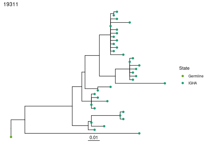
Plot trees with dowser and ggtree
Regardless of how you build trees, they are visualized in the same
manner with the plotTrees function. This will return a list of
ggplot objects in the same order as the input object. Here, we color
the tips by the isotype value because we specified that column in the
formatClones step.
Plot all of the trees:
plots_all <- dowser::plotTrees(trees, tips = "isotype", tipsize = 2)
Plot the largest tree:
plots_all[[1]]
# save a pdf of all trees
dowser::treesToPDF(plots_all,
          file = file.path("intro-lab_files", "final_data_trees.pdf"),
          nrow = 2, ncol = 2)

## png
##   2
In addition to the functions for building and visualizing trees,
dowser also implements new techniques for analyzing B cell migration
and differentiation, as well as for detecting new B cell evolution over
time. Visit the dowser website to learn
more.
SHazaM: mutational load
B cell repertoires differ in the number of mutations introduced during
somatic hypermutation (SHM). The shazam R package provides a wide
array of methods focused on the analysis of SHM, including the
reconstruction of SHM targeting models and quantification of selection
pressure.
Having identified the germline sequence (germline_alignment_d_mask) in
previous steps, we first identify the set of somatic hypermutations by
comparing the observed sequence (sequence_alignment) to the germline
sequence. observedMutations is next used to quantify the mutational
load of each sequence using either absolute counts (frequency=F) or as
a frequency (the number of mutations divided by the number of
informative positions (frequency=T). Each mutation can be defined as
either a replacement mutation (R, or non-synonymous mutation, which
changes the amino acid sequence) or a silent mutation (S, or synonymous
mutation, which does not change the amino acid sequence). R and S
mutations can be counted together (conmbine=T) or independently
(combine=F). Counting can be limited to mutations occurring within a
particular region of the sequence (for example, to focus on the V region
regionDefinition=IMGT_V) or use the whole sequence
(regionDefinition=NULL).
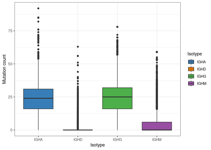
Standard ggplot commands can be used to generate boxplots to visualize
the distribution of mutation counts across sequences, which are found in
the column mu_count that observedMutations added to db.
# Calculate total mutation count, R and S combined
results@db <- observedMutations(results@db, sequenceColumn = "sequence_alignment",
                        germlineColumn = "germline_alignment_d_mask",
                        regionDefinition = NULL, frequency = F,
                        combine = T, nproc = 4)
ggplot(results@db, aes(x = isotype, y = mu_count, fill = isotype)) +
  geom_boxplot() +
  scale_fill_manual(name = "Isotype", values = IG_COLORS) +
  xlab("Isotype") + ylab("Mutation count") + theme_bw()
SHazaM: models of SHM targeting biases
SHM is a stochastic process, but does not occur uniformly across the
V(D)J sequence. Some nucleotide motifs (i.e., hot-spots) are targeted
more frequently than others (i.e., cold-spots). These intrinsic biases
are modeled using 5-mer nucleotide motifs. For each 5-mer (e.g., ATCTA),
a SHM mutability model provides the relative likelihood for the center
base (e.g., the C in ATCTA) to be mutated. As associated substitution
model provides the relative probabilities of the center base in a 5-mer
mutating to each of the other 3 bases. There are several pre-built SHM
targeting models included in shazam which have been constructed based
on experimental datasets. These include models for human and mouse, and
for both light and heavy chains. In addition, shazam provides the
createTargetingModel method to generate new SHM targeting models from
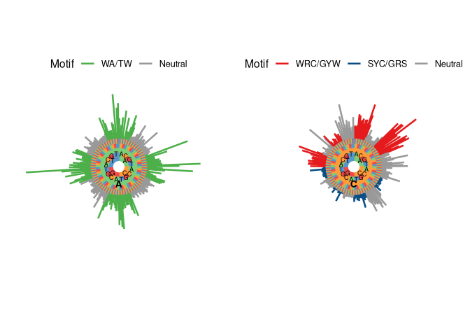
user-supplied sequencing data.  The resulting model
can be visualized as a hedgehog plot with
The resulting model
can be visualized as a hedgehog plot with plotMutability. In this
visualization, 5-mers that belong to classically-defined SHM hot-spot
motifs (e.g., WRC) are shown in red and green, cold-spot motifs in blue,
and other motifs (i.e., neutral) in grey. The bars radiating outward are
the relative mutabilities of each 5-mer. The middle circle is the
central nucleotide being targeted for SHM, here shown by a green circle
on the left plot (nucleotide A) and an orange circle on the right plot
(nucleotide C). Moving from the center of the circle outward covers the
5-mer nucleotide motif (5’ to 3’). As expected, higher relative mutation
rates are observed at hot-spot motifs.
# Build and plot SHM targeting model
m <- createTargetingModel(results@db, vCallColumn = "v_call_genotyped")

## Warning in createMutabilityMatrix(db, sub_mat, model = model, sequenceColumn =
## sequenceColumn, : Insufficient number of mutations to infer some 5-mers. Filled
## with 0.

# nucleotides: center nucleotide characters to plot
plotMutability(m, nucleotides = c("A","C"), size = 1.2)
SHazaM: quantification of selection pressure
During T-cell dependent adaptive immune responses, B cells undergo
cycles of SHM and affinity-dependent selection that leads to the
accumulation of mutations that improve their ability to bind antigens.
The ability to estimate selection pressure from sequence data is of
interest to understand the events driving physiological and pathological
immune responses. shazam incorporates the Bayesian estimation of
Antigen-driven SELectIoN (BASELINe) framework, to detect and quantify
selection pressure, based on the analysis of somatic hypermutation
patterns. Briefly, calcBaseline analyzes the observed frequency of
replacement and silent mutations normalized by their expected frequency
based on a targeting model, and generates a probability density function
(PDF) for the selection strength (∑). This PDF can be used to
statistically test for the occurrence of selection, as well as compare
selection strength across conditions. An increased frequency of R
mutations (∑ > 0) suggests positive selection, and a decreased
frequency of R mutations (∑ < 0) points towards negative selection .

positive Σ: Replacement frequency higher than expected
negative Σ: Replacement frequency lower than expected
The somatic hypermutations that are observed in clonally-related
sequences are not independent events. In order to generate a set of
independent SHM events, selection pressure analysis starts by collapsing
each clone to one representative sequence (with its associated germline)
using the function collapseClones. Next calcBaseline takes each
representative sequences and calculates the selection pressure. The
analysis can be focused on a particular region, the V region
(regionDefinition=IMGT_V) in the example below. Because selection
pressure may act differently across the BCR, we may also be interested
to evaluate the selection strength for different regions such as the
Complementary Determining Regions (CDR) or Framework Regions (FWR)
separately. Selection strength can also be calculated separately for
different isotopes or subjects. This can be done with groupbaseline,
which convolves the PDFs from individual sequences into a single PDF
representing the group of sequences (e.g., all IgG sequences). These PDF
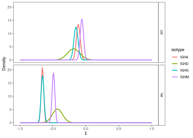
can be visualized with plot. FWR are critical to maintenance the
overall structure of the BCR and typically have a lower observed
selection strength, because mutations that alter the amino acid sequence
are often negatively selected. CDRs are the areas of the BCR that
generally bind to the antigen and may be subject to increased selection
strength, although this can depend on the point in affinity maturation
when the sequence is observed. In the example, negative selection is
observed in the FWR, and almost no selection is observed in the CDR. In
both CDR and FWR, sequences annotated with IGHM isotype show more
positive selection strength than sequences annotated with IGHG and IGHA.
# Calculate clonal consensus and selection using the BASELINe method
z <- collapseClones(results@db)
b <- calcBaseline(z, regionDefinition = IMGT_V)

## calcBaseline will calculate observed and expected mutations for clonal_sequence using clonal_germline as a reference.

## Calculating BASELINe probability density functions...

# Combine selection scores for all clones in each group
g <- groupBaseline(b, groupBy = "isotype")

## Grouping BASELINe probability density functions...
## Calculating BASELINe statistics...

# Plot probability densities for the selection pressure
plot(g, "isotype", sigmaLimits = c(-1, 1), silent = F)
SHazaM: Built in mutation models
shazam comes with several pre-built targeting models, mutation models
and sequence region definitions. They can be used to change the default
behavior of many functions. For example, mutations are usually defined
as R when they introduce any change in the amino acid sequence (NULL).
However, for some analyses, it may be useful to consider some amino acid
substitutions to be equivalent (i.e., treated as silent mutations). For
example, it is possible to define replacement mutations as only those
that introduce a change in the amino acid side chain charge
(CHARGE_MUTATIONS).
Empirical SHM Targeting Models
HH_S5F: Human heavy chain 5-mer model
HKL_S5F: Human light chain 5-mer model
MK_RS5NF: Mouse light chain 5-mer model
Mutation Definitions
NULL: Any mutation that results in an amino acid substitution is considered a replacement (R) mutation.
CHARGE_MUTATIONS: Only mutations that alter side chain charge are replacements.
HYDOPATHY_MUTATIONS: Only mutations that alter hydrophobicity class are replacements.
POLARITY_MUTATIONS: Only mutations that alter polarity are replacements.
VOLUME_MUTATIONS: Only mutations that alter volume class are replacements.
Sequence Region Definitions
NULL: Full sequence
IMGT_V: V segment broken into combined CDRs and FWRs
IMGT_V_BY_REGIONS: V segment broken into individual CDRs and FWRs