Single Cell V(D)J Analysis Tutorial
Tutorial outline:
Cloning thresholds (automatically or manually)
Calculate V gene SHM frequency (in the heavy chain)
Analyze B cell migration, differentiation, and evolution over time
Overview
This tutorial is a basic walk-through for defining B cell clonal families and building B cell lineage trees using 10x Genomics BCR (B cell receptor) sequencing data.
Knowledge of basic command line usage is assumed. Please check out the individual documentation sites for the functions detailed in this tutorial before using them on your own data.
For simplicity, this tutorial will use the Immcantation Lab Docker image which contains R Markdown notebooks and all necessary software to run this code.
You can download the current Docker image with
docker pull immcantation/lab:develFor some operating systems, it may be necessary to use super-user privileges (sudo), and/or to have Docker Desktop running before entering the previous command.
You can read more details about how to get and use the Docker container here, including how to run tutorials such as this one.
It is also possible to install the packages being used separately. Instructions are available in each package’s documentation site. See Resources.
You may also reference this page for an example pipeline script to process 10x data with Immcantation’s changeo-10x example script.
Resources:
You can email immcantation@googlegroups.com with any questions or issues.
Documentation: http://immcantation.org
Package specific documentation: pRESTO, Change-O, Alakazam, SHazaM, SCOPer, and dowser.
Source code and bug reports: https://github.com/immcantation/immcantation
Docker image for this tutorial: https://hub.docker.com/r/immcantation/lab
Source code for Immcantation tutorials: https://github.com/immcantation/immcantation/tree/master/training/
Getting started
10x BCR data and 10x GEX (gene expression) data can borrow information from each other for an improved analysis. This tutorial demonstrates a few approaches to integrating these data types along with examples on how the new information can be used.
The example files used in this tutorial are subsamples of the original 10x scRNA-seq and BCR sequencing data from Turner et al. (2020) Human germinal centres engage memory and naive B cells after influenza vaccination Nature. 586, 127–132. The study consists of blood and lymph node samples taken from a single patient at multiple time points following influenza vaccination.
We extracted a subset (~3000 cells) of single cell GEX/BCR data of
ultrasound-guided fine needle aspiration (FNA) samples of lymph nodes
for subject P05. These 3000 cells were randomly divided into two
pseudo-subjects, ensuring that each subject has distinct clones while
maintaining a similar clone size distribution. The example data is
already in the container (/home/magus/data/). If you want to, you can
download it from Zenodo
![]() .
We will use these files:
.
We will use these files:
filtered_contig.fasta and filtered_contig_annotations.csv. They are the direct Cell Ranger output files for one of the pseudo-subjects. We are going to use the Ig V(D)J sequences from this sample to show how to process V(D)J data using Immcantation.
BCR_data.tsv: B-Cell Receptor Data. Adaptive Immune Receptor Repertoire (AIRR) tsv BCRs from two pseudo-subjects, already aligned to IMGT V, D, and J genes.
GEX.data_08112023.rds: Gene Expression Data. This file contains a Seurat object with RNA-seq data already processed and annotated. Processing and annotation are not covered in this tutorial. You can learn more on these topics in Seurat’s documentation and tutorials: https://satijalab.org/seurat/articles/pbmc3k_tutorial.html
The R Markdown notebook with the code is also available in the container
(/home/magus/notebooks/10x_tutorial.Rmd).
Assign V, D, and J genes using IgBLAST
To process 10x V(D)J data, a combination of AssignGenes.py and
MakeDb.py can be used to generate a TSV file compliant with the AIRR
Community Rearrangement
schema
that incorporates annotation information provided by the Cell Ranger
pipeline. The files of filtered_contig.fasta and
filtered_contig_annotations.csv, generated by cellranger vdj,
can be found in the outs directory.
Generate AIRR Rearrangement data from the 10x V(D)J FASTA files using
the steps below (the \ just indicates a new line for visual clarity).
This step needs to be run in the command line after installing Change-O and igblast, or within the immcantation docker container. There is documentation on how to use the immcantation docker container on the Docker container section of the immcantation website. If not using the docker container, the path to the igblast executable will need to be updated to the local installation path.
# assign V, D, and J genes using IgBLAST
AssignGenes.py igblast \
   -s /home/magus/data/filtered_contig.fasta \
   -b /usr/local/share/igblast \
   --organism human --loci ig --format blast \
   --outdir results --outname BCR_data_sequences

# convert IgBLAST output to AIRR format
MakeDb.py igblast \
   -i results/BCR_data_sequences_igblast.fmt7 \
   -s /home/magus/data/filtered_contig.fasta \
   -r /usr/local/share/germlines/imgt/human/vdj/ \
   --10x /home/magus/data/filtered_contig_annotations.csv --extended

ls results
After running these commands, you should now have
BCR_data_sequences_igblast_db-pass.tsv and
BCR_data_sequences_igblast.fmt7 in your results directory.
For a full listing of what the flags mean, see the command line usage for AssignGenes.py igblast and MakeDb.py igblast. You can also read our “Using IgBLAST” which contains both commands.
The
--10x filtered_contig_annotations.csvspecifies the path of the contig annotations file generated bycellranger vdj, which can be found in the outs directory.
Please note that:
all_contig.fasta can be exchanged for filtered_contig.fasta, and all_contig_annotations.csv can be exchanged for filtered_contig_annotations.csv to use the unfiltered cellranger data outputs.
The resulting tab-delimited table overwrites the V, D and J gene assignments generated by Cell Ranger and uses those generated by IgBLAST or IMGT/HighV-QUEST instead.
To process mouse data and/or TCR data, alter the
--organismand--lociarguments toAssignGenes.pyaccordingly (e.g.,--organism mouse,--loci tcr) and use the appropriate V(D)J IMGT reference database (e.g., **imgt_mouse_TR*.fasta**)
Install and load libraries
Note that you might need to install several Bioconductor packages that
are dependencies for some of the R-based Immcantation packages with
BiocManager.
# check for ggtree, a Bioconductor package
packages <- "ggtree"

package.check <- lapply(
  packages,
  FUN = function(x) {
    if (!require(x, character.only = TRUE)) {
      install.packages(x, dependencies = TRUE)
    }
  }
)

if (!require(packages, character.only = TRUE)) {
  if (!require("BiocManager", quietly = TRUE)) {
    install.packages("BiocManager")
  }
  BiocManager::install(packages)
}
Load libraries
# load libraries
suppressPackageStartupMessages(library(airr))
suppressPackageStartupMessages(library(alakazam))
suppressPackageStartupMessages(library(dowser))
suppressPackageStartupMessages(library(dplyr))
suppressPackageStartupMessages(library(ggplot2))
suppressPackageStartupMessages(library(ggtree))
suppressPackageStartupMessages(library(scoper))
suppressPackageStartupMessages(library(Seurat))
suppressPackageStartupMessages(library(shazam))
Load in and reformat the data
Merge different samples
The preceding instructions outline the process of assigning V, D, and J
genes using IgBLAST for a single sample. In practice, each sample should
undergo individual processing following the same steps. To facilitate
the amalgamation of various samples for subsequent analysis, it is
necessary to augment the resulting table with a column labeled
sample_id (and possibly subject_id) for sample identification.
Furthermore, to ensure uniqueness across samples, sequence IDs and cell
barcodes may be modified by appending the sample ID to them. This step
has already been performed and the resulting table can be found under
/home/magus/data/BCR_data.tsv.
# read in the data
# specify the data types of non AIRR-C standard fields
# we assign integer type to the *_length fields
bcr_data <- airr::read_rearrangement(file.path("", "home", "magus", "data",
                                               "BCR_data.tsv"),
                                     aux_types = c("v_germline_length" = "i",
                                                   "d_germline_length" = "i",
                                                   "j_germline_length" = "i",
                                                   "day" = "i"))
cat(paste("There are", nrow(bcr_data),
          "rows in `bcr_data`.\n"))

## There are 6196 rows in `bcr_data`.
Check V/D/J gene call consistency
10x Genomics data can sometimes contain inconsistent gene calls where V,
J, and C genes are assigned from different immunoglobulin loci (IGH,
IGK, or IGL). This can occur particularly in cells with
chain == "Multi", but also in other cases. Usually the number of
sequences with these inconsistencies is very small. However, it is
important to remove these inconsistencies before downstream analysis.
# Filter out inconsistent sequences
bcr_data <- bcr_data %>%
  dplyr::filter(
    (grepl("^IGHV", v_call) & grepl("^IGHJ", j_call) & grepl("^IGH[MGADE]", c_gene)) |
    (grepl("^IGKV", v_call) & grepl("^IGKJ", j_call) & grepl("^IGKC", c_gene)) |
    (grepl("^IGLV", v_call) & grepl("^IGLJ", j_call) & grepl("^IGLC", c_gene))
  )
cat(paste("There are", nrow(bcr_data),
          "rows in the data after filtering V/J/C calls inconsistent with the respective locus.\n"))

## There are 6176 rows in the data after filtering V/J/C calls inconsistent with the respective locus.
Remove non-productive sequences
You may wish to subset your data to only productive sequences:
# read in the data
bcr_data <- bcr_data %>% dplyr::filter(productive)

cat(paste("There are", nrow(bcr_data), "rows in the data.\n"))

## There are 6176 rows in the data.

bcr_data %>% slice_sample(n = 5) # random examples

## # A tibble: 5 x 66
##   sequence_id                 sequence  rev_comp productive v_call d_call j_call
##   <chr>                       <chr>     <lgl>    <lgl>      <chr>  <chr>  <chr>
## 1 ACACTGATCTGTTGAG-1_contig_2 TGGGGAGG~ FALSE    TRUE       IGKV1~ <NA>   IGKJ4~
## 2 AGTAGTCAGGAATGGA-1_contig_1 AGCTCTCA~ FALSE    TRUE       IGHV3~ IGHD7~ IGHJ2~
## 3 CGGAGTCTCACTCCTG-1_contig_1 AGAGATCT~ FALSE    TRUE       IGLV1~ <NA>   IGLJ3~
## 4 TTAGGACAGAGTACAT-1_contig_2 GGAGAAGA~ FALSE    TRUE       IGKV3~ <NA>   IGKJ2~
## 5 TGAGGGAAGCCACCTG-1_contig_1 AGAGCTCT~ FALSE    TRUE       IGLV4~ <NA>   IGLJ3~
## # i 59 more variables: sequence_alignment <chr>, germline_alignment <chr>,
## #   junction <chr>, junction_aa <chr>, v_cigar <chr>, d_cigar <chr>,
## #   j_cigar <chr>, vj_in_frame <lgl>, stop_codon <lgl>, v_sequence_start <int>,
## #   v_sequence_end <int>, v_germline_start <int>, v_germline_end <int>,
## #   np1_length <int>, d_sequence_start <int>, d_sequence_end <int>,
## #   d_germline_start <int>, d_germline_end <int>, np2_length <int>,
## #   j_sequence_start <int>, j_sequence_end <int>, j_germline_start <int>, ...
Remove cells with multiple heavy chains
If your single cell data contains cells with multiple heavy chains, you need to handle it before calling clones (B cells that descend from a common naive B cell ancestor).
A simple solution is just to remove cells with multiple heavy chains from the single cell data:
# remove cells with multiple heavy chain
multi_heavy <- table(dplyr::filter(bcr_data, locus == "IGH")$cell_id)
multi_heavy_cells <- names(multi_heavy)[multi_heavy > 1]

bcr_data <- dplyr::filter(bcr_data, !cell_id %in% multi_heavy_cells)
cat(paste("There are", nrow(bcr_data),
          "rows in the data after filtering out cells with multiple heavy chains.\n"))

## There are 6160 rows in the data after filtering out cells with multiple heavy chains.
Remove cells without heavy chains
Since most of the following analyses are based on heavy chains, we remove cells with only light chains:
# split cells by heavy and light chains
heavy_cells <- dplyr::filter(bcr_data, locus == "IGH")$cell_id
light_cells <- dplyr::filter(bcr_data, locus == "IGK" | locus == "IGL")$cell_id
no_heavy_cells <- light_cells[which(!light_cells %in% heavy_cells)]

bcr_data <- dplyr::filter(bcr_data, !cell_id %in% no_heavy_cells)
cat(paste("There are", nrow(bcr_data), "rows in the data after filtering out
          cells without heavy chains."))

## There are 6160 rows in the data after filtering out
##           cells without heavy chains.
Add cell type annotations
Load gene expression Seurat object
We load the gene expression data Seurat object that has already been pre-processed and the cell types (PBMCs) have been annotation following the standard Seurat workflow.
gex_db <- readRDS(file.path("", "home", "magus", "data",
                            "GEX.data_08112023.rds"))
Inspect the data:
# Object summary
# `print` can be used to obtain a general overview of the Seurat object
# (number of features, number of samples, etc.)
print(gex_db)

## An object of class Seurat
## 19293 features across 3729 samples within 1 assay
## Active assay: RNA (19293 features, 1721 variable features)
##  1 layer present: data
##  2 dimensional reductions calculated: pca, umap
Idents reports the cell ID and identities.
# cell type annotations
head(Idents(gex_db), 1)

## subject2_FNA_d60_1_Y1_GCGACCAGTTGGAGGT-1
##                                      RMB
## Levels: RMB ABC Naive PB GC DC T B NK Monocyte
Standardize cell IDs
Both of the example datasets have been processed separately and use slightly different cell identifiers. To consolidate the data into one object, we need to standardize the cell identifiers. This step could be different or even not necessary with other datasets.
# make cell IDs in BCR match those in Seurat object
bcr_data$cell_id_unique <- paste0(bcr_data$sample_id, "_", bcr_data$cell_id)
bcr_data$cell_id_unique[1]

## [1] "subject2_FNA_d60_1_Y1_GCGACCAGTTGGAGGT-1"
In addition, the cells in both datasets are not presented in the same order.
# first id in the BCR data
bcr_data$cell_id_unique[1]

## [1] "subject2_FNA_d60_1_Y1_GCGACCAGTTGGAGGT-1"

# first id in the GEX data
Cells(gex_db)[1]

## [1] "subject2_FNA_d60_1_Y1_GCGACCAGTTGGAGGT-1"
Having common cell identifiers, we can bring BCR data into the Seurat
object, or the GEX and annotation data from the Seurat object into the
BCR table, by matching cell_id_unique.
Match GEX and BCR cell ids
We perform a match step to identify the GEX data in the BCR object.
The vector match.index will contain the positions of the BCR sequences
in the GEX data.
# match indices to find the position of the BCR cells in the GEX data
# different from finding the position of the GEX cells in the BCR data!
match.index <- match(bcr_data$cell_id_unique, Cells(gex_db))
Some BCRs don’t have GEX information. This can happen, for example, if the cell for which BCRs are covered didn’t pass the GEX processing and quality control thresholds. The proportion of BCRs that do not have GEX information is:
# what proportion of BCRs don’t have GEX information?
mean(is.na(match.index))

## [1] 0.08198052
Transfer cell type annotations into the BCR data
The GEX cell type annotations can be added as additional columns in the BCR table:
# add annotations to BCR data
cell.annotation <- as.character(Idents(gex_db))
bcr_data$gex_annotation <-
  unlist(lapply(match.index, function(x) {
    ifelse(is.na(x), NA, cell.annotation[x])
  }))

bcr_data$gex_annotation[1:5]

## [1] "RMB" NA    "GC"  "GC"  "RMB"
Remove cells without GEX data
In this tutorial, we exclude cells from BCR data that lack corresponding partners in GEX data before conducting clonal analysis. This step deviates from the usual practice.
# remove cells that didn’t match
bcr_data <- dplyr::filter(bcr_data, !is.na(gex_annotation))
Clonal analysis
Goal: Partition (cluster) sequences into clonally related lineages. Each lineage is a group of sequences that came from the same original naive cell.
Summary of the key steps:
Determine clonal clustering threshold: sequences which are under this cut-off are clonally related.
Assign clonal groups: add an annotation (
clone_id) that can be used to identify a group of sequences that came from the same original naive cell.Reconstruct germline sequences: figure out the germline sequence of the common ancestor, before mutations are introduced during clonal expansion and SMH.
Identify clonal threshold
Manual
Hierarchical clustering is a widely used distance-based method for
identify clonally related sequences. An implementation of the
hierarchical clustering approach is provided via the
hierarchicalClones function in the
SCOPer R package.
It is important to determine an appropriate threshold for trimming the
hierarchical clustering into B cell clones before using this method. The
ideal threshold for separating clonal groups is the value that separates
the two modes of the nearest-neighbor distance distribution. The
nearest-neighbor distance distribution can be generated by using the
distToNearest function in the
SHazaM R package.
We define a clonal threshold only using the heavy chain locus, so we need to filter the dataset for the “IGH” locus. Clonal groups should be defined within one subject:
dist_nearest <- distToNearest(dplyr::filter(bcr_data,
                                            locus == "IGH",
                                            subject_id == "subject1"),
                              cellIdColumn="cell_id")

## Running in single-cell mode.

# generate Hamming distance histogram
p1 <- ggplot(subset(dist_nearest, !is.na(dist_nearest)),
             aes(x = dist_nearest)) +
        geom_histogram(color = "white", binwidth = 0.02) +
        labs(x = "Hamming distance", y = "Count") +
        scale_x_continuous(breaks = seq(0, 1, 0.1)) +
        theme_bw() +
        theme(axis.title = element_text(size = 18))

plot(p1)
The resulting distribution is often bimodal, with the first mode representing sequences with clonal relatives in the dataset and the second mode representing singletons. We can inspect the plot of nearest-neighbor distance distribution generated above to manually select a threshold to separates the two modes of the nearest-neighbor distance distribution.
This procedure should be repeated for all subjects in the dataset. A mean or median of the identified threshold can then be used as the final threshold for defining clones. We recommended to always inspect all the distance histograms to verify that the threshold selected is reasonable for all subjects.
For further details regarding inferring an appropriate threshold for the hierarchical clustering method, see the Distance to Nearest Neighbor vignette in the SHazaM package.
Automatic
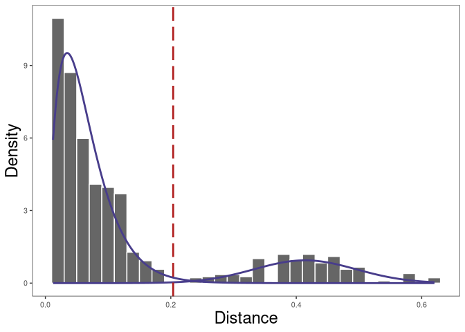
The figure shows the distance-to-nearest distribution for the repertoire. Typically, the distribution is bimodal. The first mode (on the left) represents sequences that have at least one clonal relative in the dataset, while the second mode (on the right) is representative of the sequences that do not have any clonal relatives in the data (sometimes called “singletons”). A reasonable threshold will separate these two modes of the distribution.
The threshold itself can be also found using the automatic
findThreshold function. There are different ways to find the threshold
and details can also be found in the Distance to Nearest Neighbor
vignette
in the shazam package.
A robust way that we recommend is to use the nearest-neighbor distance of inter (between) clones as the background and select the threshold based on the specificity of this background distribution.
# find threshold for cloning automatically
threshold_output <- shazam::findThreshold(dist_nearest$dist_nearest,
                                          method = "gmm", model = "gamma-norm",
                                          cutoff = "user", spc = 0.995)
threshold <- threshold_output@threshold
threshold

## [1] 0.2037778

plot(threshold_output, binwidth = 0.02, silent = TRUE) +
  theme(axis.title = element_text(size = 18))
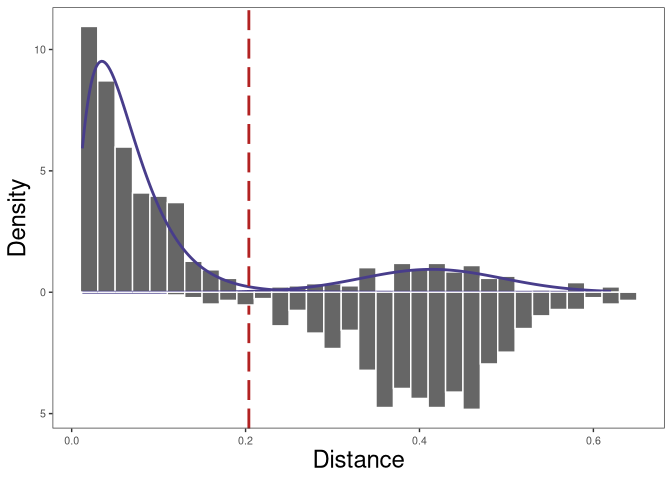
The nearest-neighbor distance distribution is not always bimodal. In this case, if the data have multiple subjects, we can calculate the nearest neighbor distances across subjects to initialize the Gaussian fit parameters of the nearest-neighbor distance of inter (between) clones distribution.
The nearest neighbor distances across subjects can be calculated by
specifying the parameter cross in the function distToNearest. And
then when we call function findThreshold, Gaussian fit parameters can
be initialized by setting parameter
cross = dist_crossSubj$cross_dist_nearest.
In the above data, there are two subjects. We will want to make make
sure that the cross subject distToNearest values are valid. To
calculate this do the following:
# calculate cross subjects distribution of distance to nearest
dist_crossSubj <- distToNearest(dplyr::filter(bcr_data, locus == "IGH"),
                                nproc = 1, cross = "subject_id",
                                cellIdColumn="cell_id")

## Running in single-cell mode.

# find threshold for cloning automatically and initialize the Gaussian fit
# parameters of the nearest-neighbor

# distance of inter (between) clones using cross subjects distribution of distance to nearest
threshold_output <- shazam::findThreshold(dist_nearest$dist_nearest,
                                          method = "gmm", model = "gamma-norm",
                                          cross = dist_crossSubj$cross_dist_nearest,
                                          cutoff = "user", spc = 0.995)
threshold_withcross <- threshold_output@threshold
threshold_withcross

## [1] 0.2037778

# plot the threshold along the density plot
plot(threshold_output, binwidth = 0.02,
     cross = dist_crossSubj$cross_dist_nearest, silent = TRUE) +
  theme(axis.title = element_text(size = 18))
In the plot above, the top plot is the nearest-neighbor distance distribution within Subj1, and the bottom plot is the nearest neighbor distances across Subj1 and Subj2.
Define clonal groups
Once a threshold is decided, we perform the clonal assignment. At the
end of this step, the BCR table will have an additional column
(clone_id) that provides an identifier for each sequence to indicate
which clone it belongs to (i.e., sequences that have the same identifier
are clonally-related). Note that these identifiers are only unique to
the dataset used to carry out the clonal assignments.
The hierarchicalClones function in SCOPer package can be used to
call clones using single cell mode:
# call clones using hierarchicalClones
results <- hierarchicalClones(bcr_data,
                              cell_id = "cell_id_unique",
                              threshold = threshold,
                              only_heavy = TRUE, split_light = FALSE,
                              summarize_clones = FALSE,
                              fields = "subject_id")

## Running defineClonesScoper in single cell mode
hierarchicalClones clusters B receptor sequences based on junction
region sequence similarity within partitions that share the same V gene,
J gene, and junction length, thus allowing for ambiguous V or J gene
annotations. By setting it up the cell_id parameter,
hierarchicalClones will run in single cell mode with paired-chain
sequences. With only_heavy = TRUE and split_light = TRUE, grouping
should be done by using IGH only and inferred clones should be split by
the light/short chain (IGK and IGL) following heavy/long chain
clustering.
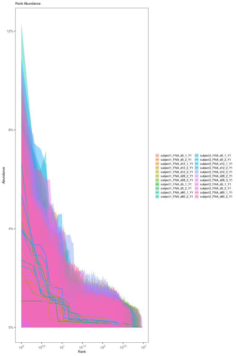
Visualize clonal abundance
After calling clones, a clonal abundance distribution can be displayed. To estimate the clonal abundance, we will select only the heavy chains:
# calculate and plot the rank-abundance curve
abund <- estimateAbundance(dplyr::filter(results, locus == "IGH"),
                           group = "sample_id", nboot = 100)

## Adding missing grouping variables: `subject_id`

abund_plot <- plot(abund, silent=T)
abund_plot
# plot by sample_id
abund_plot + facet_wrap("sample_id", ncol = 3)
 Most real
datasets, will have most clones of size 1 (one sequence). In this
tutorial, we processed data to remove most of singleton clone and we
don’t see the much higher peak at 1 that we would normally expect.
Most real
datasets, will have most clones of size 1 (one sequence). In this
tutorial, we processed data to remove most of singleton clone and we
don’t see the much higher peak at 1 that we would normally expect.
# get clone sizes using dplyr functions
clone_sizes <- countClones(dplyr::filter(results, locus == "IGH"),
                           groups = "sample_id")

## Adding missing grouping variables: `subject_id`

# plot cells per clone
ggplot(clone_sizes, aes(x = seq_count)) +
  geom_bar() +
  facet_wrap("sample_id", ncol = 3) +
  labs(x = "Sequences per clone") +
  theme_bw()

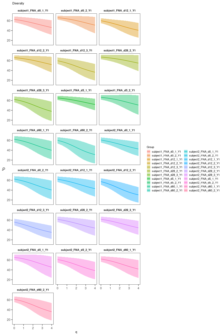
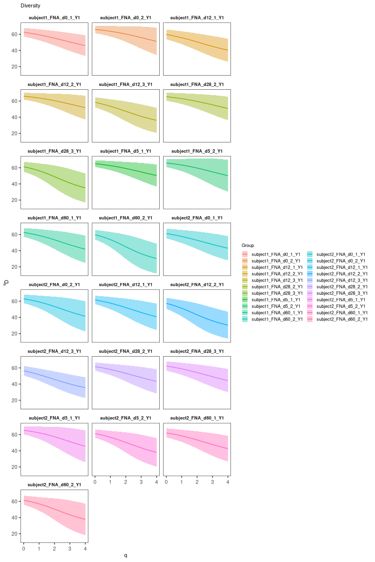
Visualize clonal diversity
The clonal diversity can also be displayed. To estimate the clonal diversity, we will also select only the heavy chains:
# calculate and plot the rank-abundance curve
div <- alphaDiversity(dplyr::filter(results, locus == "IGH"),
                      group = "sample_id", nboot = 100)

## Adding missing grouping variables: `subject_id`

plot(div, silent = TRUE) + facet_wrap("sample_id", ncol = 3)
Create germlines
The goal is to reconstruct the sequence of the unmutated ancestor of
each clone using a reference database of known alleles
(IMGT), before building B cell lineage trees. Due
to the challenging nature of accurately inferring the D region and the
junction region for BCR sequences, this region is masked with N. Note
that occasionally errors are thrown for some clones - this is typical
and usually results in those clones being excluded.
In the example below, we read in the IMGT germline references from our Docker container. If you’re using a local installation, you can download the most up-to-date reference genome by cloning the Immcantation repository and running the script:
# Retrieve reference genome with the script fetch_imgtdb.sh.
# It will create directories where it is run
git clone https://bitbucket.org/kleinstein/immcantation.git
./immcantation/scripts/fetch_imgtdb.sh
And passing "human/vdj/" to the readIMGT function.
# read in IMGT data if downloaded on your own (above)
# and update `dir` to use the path to your `human/vdj` folder
# references <- readIMGT(dir = "human/vdj/")

# read in IMGT files in the Docker container
references <- readIMGT(dir = "/usr/local/share/germlines/imgt/human/vdj")

## [1] "Read in 1305 from 17 fasta files"

# reconstruct germlines
results <- createGermlines(results, references, fields = "subject_id",
                           nproc = 1)
Calculate V gene SHM frequency
Basic mutational load calculations can be performed by the function
observedMutations in the
SHazaM R package:
# this is typically only done on heavy chains, but can also be done on light chains
results_heavy <- dplyr::filter(results, locus == "IGH")

# calculate SHM frequency in the V gene
data_mut <-
  shazam::observedMutations(results_heavy,
                            sequenceColumn = "sequence_alignment",
                            germlineColumn = "germline_alignment_d_mask",
                            regionDefinition = IMGT_V,
                            frequency = TRUE,
                            combine = TRUE,
                            nproc = 1)
The plot below shows the distribution of median mutation frequency of clones:
# calculate the median mutation frequency of a clone
mut_freq_clone <- data_mut %>%
                    dplyr::group_by(clone_id) %>%
                    dplyr::summarize(median_mut_freq = median(mu_freq))

ggplot(mut_freq_clone, aes(median_mut_freq)) +
  geom_histogram(binwidth = 0.005) +
  theme_bw() + theme(axis.title = element_text(size = 18))

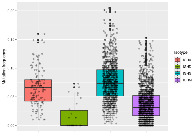
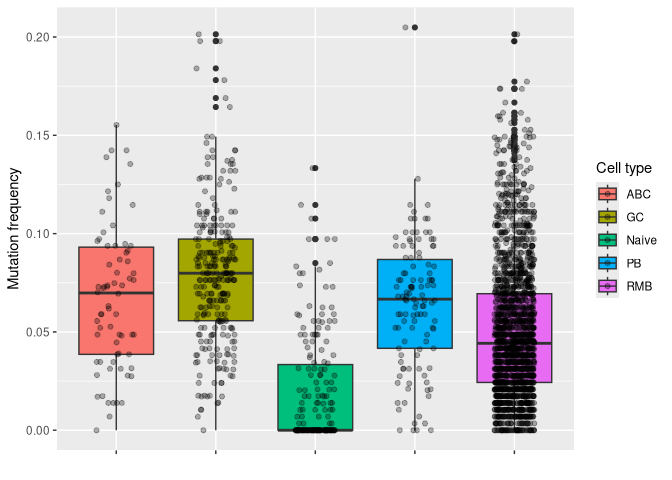
The plots below show the distribution of mutation frequency of cells by subject, isotype and cell type respectively:
# plotting mu_freq by subject_id
ggplot(data_mut, aes(y = mu_freq, x = subject_id, fill = subject_id)) +
  geom_boxplot() +
  geom_jitter(width = 0.2, alpha = 0.3) +
  labs(x = "", y = "Mutation frequency", fill = "subject_id") +
  theme(axis.text.x = element_blank())

# plotting mu_freq by isotype
ggplot(data_mut, aes(y = mu_freq, x = c_gene, fill = c_gene)) +
  geom_boxplot() +
  geom_jitter(width = 0.2, alpha = 0.3) +
  labs(x = "", y = "Mutation frequency", fill = "Isotype") +
  theme(axis.text.x = element_blank())
# plotting mu_freq by cell type
ggplot(data_mut, aes(y = mu_freq, x = gex_annotation, fill = gex_annotation)) +
  geom_boxplot() +
  geom_jitter(width = 0.2, alpha = 0.3) +
  labs(x = "", y = "Mutation frequency", fill = "Cell type") +
  theme(axis.text.x = element_blank())
Build and visualize trees
Steps:
Formatting clones
Tree building
Visualize trees
Reconstruct intermediate sequences
Format clones with dowser
In the rearrangement table, each row corresponds to a sequence, and each
column is information about that sequence. We will create a new data
structure, where each row is a clonal cluster, and each column is
information about that clonal cluster. The function formatClones
performs this processing and has options that are relevant to determine
how the trees can be built and visualized. For example, traits
determines the columns from the rearrangement data that will be included
in the clones object, and will also be used to determine the
uniqueness of the sequences, so they are not collapsed.
# make clone objects with aligned, processed sequences
# collapse identical sequences unless differ by trait
# add up duplicate_count column for collapsed sequences
# store day, gex_annotation
# discard clones with < 5 distinct sequences
clones <- formatClones(results,
                       traits = c("day", "gex_annotation"),
                       num_fields = c("duplicate_count"), minseq = 5, nproc = 1)

head(clones)

## # A tibble: 6 x 4
##   clone_id data       locus  seqs
##   <chr>    <list>     <chr> <int>
## 1 196      <airrClon> IGH      14
## 2 506      <airrClon> IGH      14
## 3 656      <airrClon> IGH      14
## 4 244      <airrClon> IGH      12
## 5 515      <airrClon> IGH      12
## 6 568      <airrClon> IGH      12
Additionally, if there is paired heavy and light chain data, you can
format the clones such that the paired data is used in building trees.
There is an additional step that occurs before the formatClones step
in this situation. In order for the trees to best use the addition of
light chain information, we will need to assign clone_subgroups using
dowser’s function resolveLightChains. This group cells within a clone
based on the light chain V and J gene and assign a subgroup to each
sequence. Then, in the formatClones step, specify chain="HL".
## Warning in formatClones(comb, chain = "HL", traits = c("day",
## "gex_annotation"), : 2 sequence(s) with an inframe stop codon were removed. If
## you want to keep these sequences use the option filterstop=FALSE.

## # A tibble: 6 x 4
##   clone_id data       locus    seqs
##   <chr>    <list>     <chr>   <int>
## 1 196      <airrClon> IGH,IGL    15
## 2 506      <airrClon> IGH,IGK    14
## 3 656      <airrClon> IGH,IGL    14
## 4 244      <airrClon> IGH,IGK    12
## 5 515      <airrClon> IGH,IGK    12
## 6 568      <airrClon> IGH,IGK    12
Build trees with dowser
Dowser offers multiple ways to build B cell phylogenetic trees. These
differ by the method used to estimate tree topology and branch lengths
(e.g. maximum parsimony and maximum likelihood) and implementation
(IgPhyML, PHYLIP, RAxML, or R packages ape and phangorn). Each
method has pros and cons.
Maximum parsimony
This is the oldest method and very popular. It tries to minimize the number of mutations from the germline to each of the tips. It can produce misleading results when parallel mutations are present.
There are two options for maximum parsimony trees. The first uses phangorn:
trees <- getTrees(clones, nproc = 1)
head(trees)

## # A tibble: 6 x 5
##   clone_id data       locus    seqs trees
##   <chr>    <list>     <chr>   <int> <list>
## 1 196      <airrClon> IGH,IGL    15 <phylo>
## 2 506      <airrClon> IGH,IGK    14 <phylo>
## 3 656      <airrClon> IGH,IGL    14 <phylo>
## 4 244      <airrClon> IGH,IGK    12 <phylo>
## 5 515      <airrClon> IGH,IGK    12 <phylo>
## 6 568      <airrClon> IGH,IGK    12 <phylo>
And the second uses dnapars (PHYLIP):
# the executable path is the location of the executable in the Docker container
trees <- getTrees(clones, build = "dnapars",
                  exec = "/usr/local/bin/dnapars", nproc = 1)

head(trees)

## # A tibble: 6 x 5
##   clone_id data       locus    seqs trees
##   <chr>    <list>     <chr>   <int> <list>
## 1 196      <airrClon> IGH,IGL    15 <phylo>
## 2 506      <airrClon> IGH,IGK    14 <phylo>
## 3 656      <airrClon> IGH,IGL    14 <phylo>
## 4 244      <airrClon> IGH,IGK    12 <phylo>
## 5 515      <airrClon> IGH,IGK    12 <phylo>
## 6 568      <airrClon> IGH,IGK    12 <phylo>
Standard maximum likelihood trees
These methods model each sequence separately. Use a markov model of the mutation process and try to find the tree, not the branch lengths, that maximizes the likelihood of seen data.
There are several options for standard maximum likelihood trees. The first uses pml (phangorn):
trees <- getTrees(clones, build = "pml", nproc = 1)
head(trees)

## # A tibble: 6 x 5
##   clone_id data       locus    seqs trees
##   <chr>    <list>     <chr>   <int> <list>
## 1 196      <airrClon> IGH,IGL    15 <phylo>
## 2 506      <airrClon> IGH,IGK    14 <phylo>
## 3 656      <airrClon> IGH,IGL    14 <phylo>
## 4 244      <airrClon> IGH,IGK    12 <phylo>
## 5 515      <airrClon> IGH,IGK    12 <phylo>
## 6 568      <airrClon> IGH,IGK    12 <phylo>
The second uses dnaml (PHYLIP):
# the executable path is the location of the executable in the Docker container
trees <- getTrees(clones, build = "dnaml",
                  exec = "/usr/local/bin/dnaml", nproc = 1)
And the third uses RAxML (RAxML-ng):
# the executable path is the location of the executable in the Docker container
trees <- getTrees(clones, build = "raxml",
                  exec = "/usr/local/bin/raxml-ng", nproc = 1)
B cell specific maximum likelihood
This is similar to the standard maximum likelihood, but incorporates SHM specific mutation biases into the tree building:
# B cell specific maximum likelihood with IgPhyML
# the executable path is the location of the executable in the Docker container
trees <- getTrees(clones, build = "igphyml",
                  exec = "/usr/local/share/igphyml/src/igphyml", nproc = 1)
In addition to standard and B cell specific maximum likelihood, dowser
offers partitioned maximum likelihood approaches for RAxML and
IgPhyML. This approach should only be used when there is paired heavy
and light chain data, not just heavy chain data because both methods
will partition on the heavy chain and light chains separately.
# RAxML
trees <- getTrees(clones, build = "raxml",
                  exec = "/usr/local/bin/raxml-ng",
                  partition = "scaled", nproc = 1)

# IgPhML
trees <- getTrees(clones, build = "igphyml",
                  exec = "/usr/local/share/igphyml/src/igphyml",
                  partition = "hl", nproc = 1)
Plot trees with dowser and ggtree
Regardless of how you build trees, they are visualized in the same
manner with the plotTrees function. This will return a list of
ggplot objects in the same order as the input object. Here, we color
the tips by the day value because we specified that column in the
formatClones step.
Plot all of the trees:
plots_all <- plotTrees(trees, tips = "day", tipsize = 2)
Plot the largest tree:
plots_all[[1]]
# save a pdf of all trees
dir.create("results/dowser_tutorial/", recursive = TRUE)

## Warning in dir.create("results/dowser_tutorial/", recursive = TRUE):
## 'results/dowser_tutorial' already exists

treesToPDF(plots_all,
           file = file.path("results", "dowser_tutorial","final_data_trees.pdf"),
           nrow = 2, ncol = 2
          )

## png
##   2
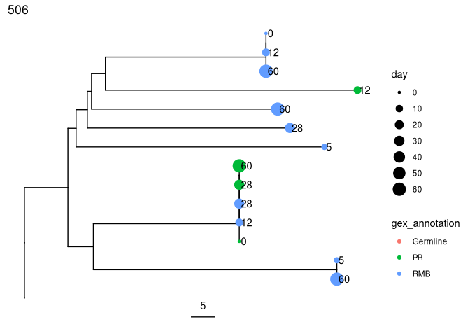
Making more informative tree plots
Plot trees so that tips are colored by cell type, scaled by sample day, and labelled by isotype:
# Scale branches to mutations rather than mutations/site
trees <- scaleBranches(trees)

# Make fancy tree plot of second largest tree
plots_all <- plotTrees(trees, scale = 5)[[2]] +
               geom_tippoint(aes(color = gex_annotation, size = day)) +
               geom_tiplab(aes(label = day), offset = 0.002)

print(plots_all)
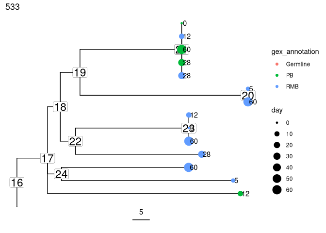
Reconstruct intermediate sequences
Sequences of intermediate nodes are automatically reconstructed during
the tree build process. To retrieve them, first plot the node numbers
for each node. The function collapseNodes can help clean up the tree
plots.
Get the predicted intermediate sequence at an internal node in the second largest tree (dots represent IMGT gaps):
# collapse nodes with identical sequences
trees <- collapseNodes(trees)

# node_nums = TRUE labels each internal node
plots_all <- plotTrees(trees, node_nums = TRUE, labelsize = 6, scale = 5)[[2]] +
               geom_tippoint(aes(color = gex_annotation, size = day)) +
               geom_tiplab(aes(label = day), offset = 0.002)

print(plots_all)

# get sequence at node 5 for the second clone_id in trees
getNodeSeq(trees, clone = trees$clone_id[2], node = 5)

##                                                                                                                                                                                                                                                                                                                                                                                                            IGH
## "CAGGTTCAACTGGTGCAGTCTGGACCT...GAGGTGAAGATGCCTGGGGCCTCAGTGGAGGTCTCCTGCGAGGCTTCTGGTTACACCTTT............TCCACCTCTGGTATCAGCTGGGTGCGACAGGCCCCTGGACAAGGGCTTGAGTGGATGGGATGGATCAGCGATGAC......AATGGTTACACAACGTATGCAGAGAATTTCCAG...GGCAGAGTCACCATGACCACAGACACATCCACAAAAACAGCCTATATGGAGCTGAGGAGGCTGAGATCTGACGACACGGCCGTGTATTATTGTGCGAGAGATGGCCAATGGGGGAGCCTCACTGGGGCGAGTTTTGACTACTGGGGCCAGGGAACCCTGGTCACCGTCTCCTCAGNN"
##                                                                                                                                                                                                                                                                                                                                                                                                            IGK
##                         "GACATCCAGATGACCCAGTCTCCATCCTCCCTGTCTGCCTCTCTAGGCGACAGAGTCACCATCACTTGCCGGGCAAGTCAGAGCATT..................AGCACCTTTTTAAATTGGTATCAGCTGAAACCAGGGAAAGCCCCTAAACTCCTGATCTATGATGCC.....................TCCAGTTTGCAAAGTGGGGTCCCA...TCAAGGTTCAGTGGCAGTGGA......TCTGGGACAGATTTCACTCTCTCCATCAGAAATCTGCAACCTGAAGATTTTGCAACTTACTACTGTCAACAGAGTTACACTATCCCTCGGACGTTCGGCCAAGGGACCAAGGTGGAAATCAAACNN"
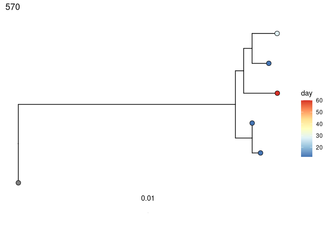
Test for measurable evolution
Perform root-to-tip regression on each tree to detect if later-sampled timepoints are more diverged from the germline:
# correlation test
trees <- correlationTest(trees, time = "day", nproc = 1)

# remove trees with one timepoint, order by p value
trees <- dplyr::filter(trees, !is.na(p))
trees <- trees[order(trees$p), ]

# coloring tips by sample day
plots_time <- plotTrees(trees)
plots_time <- lapply(plots_time, function(x) {
  x +
    geom_tippoint(aes(fill = day), shape = 21, size = 3) +
    scale_fill_distiller(palette = "RdYlBu")
})

dplyr::select(trees, clone_id, slope, correlation, p)

## # A tibble: 35 x 4
##    clone_id  slope correlation      p
##    <chr>     <dbl>       <dbl>  <dbl>
##  1 570      0.0452       0.711 0.0969
##  2 699      0.120        0.876 0.164
##  3 513      0.277        0.827 0.192
##  4 209      0.0630       0.468 0.228
##  5 1122     0.708        0.578 0.232
##  6 1118     0.489        0.444 0.249
##  7 196      0.307        0.770 0.255
##  8 573      0.0830       0.329 0.261
##  9 183      0.169        0.300 0.269
## 10 363      2.57         0.833 0.332
## # i 25 more rows

print(plots_time[[1]])
# save all trees to a pdf file
treesToPDF(plots_time,
           file = file.path("results", "dowser_tutorial", "time_data_trees.pdf"))

## png
##   2
Analyze B cell migration, differentiation, and evolution over time
In addition to the functions for building and visualizing trees,
dowser also implements new techniques for analyzing B cell migration
and differentiation, as well as for detecting new B cell evolution over
time. These are more advanced topics detailed on the dowser
website.
If you have data from different tissues, B cell subtypes, and/or isotypes and want to use lineage trees to study the pattern of those traits along lineage trees, check out the discrete trait vignette.
If you have data from multiple timepoints from the same subject and want to determine if B cell lineages are evolving over the sampled interval, check out the measurable evolution vignette.
For more advanced tree visualization, check out the plotting trees vignette.
Run a start-to-finish Immcantation workflow
The most common BCR and TCR repertoire analysis steps are implemented in the nf-core/airrflow workflow. This workflow is particularly useful for analyzing a large amount of samples in parallel. To know more about the workflow, check out the nf-core/airrflow documentation. The documentation includes a single-cell tutorial that guides you through the steps of running the workflow for single-cell datasets.